Section outline

    • 1. Motion with constant acceleration

      This program shows motion (along straight line) with constant acceleration as a function of initial velocity and acceleration. You can trace instantaneous velocity, position and displacement of a moving object.

      RUN

      2. Projectile motion

      This programs shows projectile motion as a function of initial velocity and launch angle. You can change these parameters using proper controls. Instantaneous velocity and acceleration (and their components) are displayed.

      RUN

      3. Work done by variable force

      The program illustrates calculation of the work done by a variable force. In program the area under the curve is divided into a number of narrow strips. It permits to take the force as being reasonably constant over that interval. Using proper control you can make better approximation by reducing the strip width (increasing number of strips) In the limit, the number of strips becomes very large and the area of stripes is very close to the are under F(x) curve (integral).

      RUN

      4. One dimensional collisions

      This program illustrates one dimensional collision between two balls. You can adjust initial velocity of colliding balls, their mass m and coefficient of restitution.

      RUN

      5. Two dimensional collisions

      This program shows two hard balls colliding, one moving, one at rest. You can adjust initial velocity of the striking ball, ratio of masses and impact parameter.

      RUN

    • 6. Simple harmonic motion

      This program illustrates a motion of a mass suspended on a spring. You can adjust spring constant k, mass m and the amplitude of the motion. Watch the changes of displacement, velocity, kinetic energy, potential energy, and total energy.

      RUN

      7. Damped oscillations

      Watch simple pendulum motion as a function of pendulum length, motion amplitude, and damping constant. You can change option to critical damping or aperiodic motion.

      RUN

      8. Superposition of waves

      This program displays a result of superposition of two transverse waves as a function of amplitude ratio and phase shift. Additionally you can watch standing waves and beats.

      RUN

      9. Doppler effect

      The program shows Doppler effect for sound waves in the case when source and receiver move either directly toward or directly away from each other, 'at speeds less than the speed of sound. You can change speed of the source and receiver, their direction of motion as well as source frequency.

      RUN

    • 10. Maxwell speed distribution

      The program plots the Maxwell speed distribution for a given temperature. You can compare plots generated for two selected temperatures.

      RUN

      11. Gas diffusion

      The program illustrates mixing of two gases, initially placed in two containers, as a function of the temperature. In the program you can trace actual concentration of gases and molecules speed distribution compared with the Maxwell speed distribution.

      RUN

    • 12. Electric field

      The program shows electric field lines and electric potential due to given static configuration of point 'charges. You can select particular charge configuration (e.g. dipole) or create your own charge arrangement.

      RUN

      13. Motion of a charged particle in magnetic field

      This program shows charged particle path in uniform magnetic field B. You can adjust magnitude of magnetic field B, particle’s velocity v, and angle between v and B.

      RUN

      14. Electromagnetic wave model

      This program illustrates plane polarized electromagnetic wave, which propagates in Y direction. The electric field vectors E, are parallel to the Z axis, whereas the vectors of the magnetic field B, are parallel to the X axis. You can adjust wave lenght and amplitude of the fields.

      RUN

      15. RLC series circuit

      This program simulates voltage drops across each element of the circuit R, L, C in comparision with applied voltage U(t) and the current I(t). The circuitt parameters: R, L, C and a frequency f of applied voltage may be changed with the sliders. Particularly, you can adjust either the frequency f of the source or natural frequency of the circuit (by changing L and C) to reach the resonance state.

      RUN

    • 16. Reflection and refraction of light

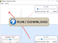
      This program illustrates the direction of the incident, reflected, and refracted rays at a flat and smooth interface surface between two materials in terms of the angle of incidence and refractive indexes n1, n2.
      RUN

      17. Lenses

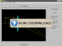
      The program illustrates graphic construction of images formed by converging and diverging lenses. Using proper control you can change position of lens and object. You can also change focal length.
      RUN

      18. Light interference

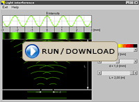
      Watch interference of two coherent light waves resulting from sending a wave through two very narrow slits (Young`s interference experiment). You can change a distance between slits, wavelength, and a distance from slits to screen.
      RUN

      19. Single-slit diffraction

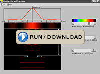
      The program displays the diffraction pattern of plane waves of light that are diffracted by a single slit. You can change a width of a slit, wavelength, and a distance from slit to screen.
      RUN

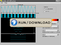
      20. Double-slit diffraction

      The program displays the diffraction pattern of plane waves of light that are diffracted by two slits. You can change a distance between slits, wavelength, a width of a slits, and a distance from slits to the screen.
      RUN

    • 21. Black body radiation

      The program plots blackbody radiation spectrum for a given temperature. You can compare plots generated for two selected temperatures.

      RUN

      22. Radioactive decay

      The program illustrates spontaneous transformation of radioactive nuclide into a different nuclide. You can watch how the number of radioactive nuclei in the sample is changing with time. You can also adjust a half-life of a radionuclide.

      RUN

      23. Photoelectric effect

      This programm visualizes the photoelectric effect experiment with photocell circuit. In program, you can adjust a voltage placed across the electrodes of photocell, light intensity, and light frequency (in the visible and ultraviolet range).

      RUN

      24. Electron wavefunctions

      Electron wavefunctions (satisfying the Schrodinger equation for the hydrogen atom) depend on the quantum numbers n, l, m. The physical interpretation of a particle wavefunction was first given by Max Born. He proposed that its square modulus can be interpreted as a probability density for finding the particle at a particular location at a particular time. This program plots (for selected quantum numbers n, l, m) the radial part of hydrogen atom, the radial and angular probability distribution function, and the visualization of hydrogen atomic orbitals in two dimensions.

      RUN